SEO & Data: A Match Made In Heaven
Professional SEO specialists possess very broad skills in everything from coding to copywriting and, crucially, in using data!
In particular those working on big websites will often find themselves spending huge amounts of time using Excel or Google Sheets to analyse, edit and optimise data.
So just learning some basic formulas and functions can take your SEO game to the next level.

The aim of this article is to showcase some pretty basic but effective data tricks, formulas and functions that can be incredibly powerful when applied to SEO tasks.
It doesn’t matter whether it’s Excel or Google Sheets, these SEO data tips are huge time savers and allow you to achieve excellent results for common SEO tasks, with absolute efficiency.
I may produce another article to show some of the more complex formulas and reports I use for my clients, but these Excel SEO tips are very much aimed at beginners who are looking to improve their SEO skills by using data effectively.
There are no limits to the number of tasks you can use these data tips for. Just picking them up now will make life so much easier when a challenge inevitably comes up.
What Data?!
Before I go any further I should clarify that I’m not talking about personal data here, I’m talking entirely about website data or about analytics data.
To be even more explicit, I’m mostly talking about all of the data extracted from websites using crawling tools such as Screaming Frog.
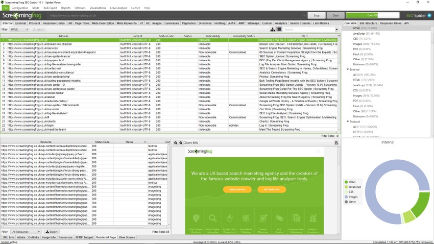
Additionally, there is a huge amount of reporting data from sources such as Google Analytics, Google Search Console and SEO tools such as Ahrefs, that is used to inspire and action the granular optimisation of pages.
You can also read my article on using Google Analytics data to optimise your site to help you with some of the applications of these formulas.
But before I begin, just a quick word about the typical type of SEO data you will mostly be pulling into Excel sheets or Google docs.
I’m going to continue using Screaming Frog as the default data supplier, since it’s the most commonly used tool by SEOs, but crawlers will typically return the same types of data.
What Data Can You Get From Screaming Frog?
Absolutely loads! Screaming Frog pulls a comprehensive list of data from a website allowing you to export and view the data in any way you wish.
Here is a brief list of some of the important data you can retrieve from a Screaming Frog crawl:
- All Website URLs
- Meta Titles
- Meta Title Lengths
- H1s-H6s
- Meta Descriptions
- Meta Description Lengths
- Status Codes (Find Error 4XX/5XX Pages)
- Redirect Chains
- Crawl Depths
- Inlinks
- Outlinks
- Directive Tags (Canonicals/Noindex)
- Images (Inc. Sizes)
The list is endless.
Conducting an SEO project, regardless of length will most often require you to export large amounts of data to fully complete the task at hand.
These tips and tricks will allow you to handle large amounts of data effectively and efficiently, enabling you to implement great traffic-boosting initiatives.
So without further ado, here are my top 7 recommended data tips and tricks for SEO….
1. The VLookup Formula

Without a doubt one of the biggest timesavers is the VLookup function.
The VLookup allows you to take two sets of data that share a common value and pull through a unique set of values from one of those sheets into your main sheet.
In a nutshell, it allows you to take the data from another file and add it to the master spreadsheet you are producing without needing to find, copy and paste.
Reading about VLookups can make it sound more complex than it is so I will outline an example…
When Would You Use A VLookup?
There are loads of scenarios where you would use a VLookup formula, but here is a common example of when it is used in SEO to highlight its purpose.
Say I am conducting a website content audit, I want the end result to show a list of URLs and various attributes relevant to each URL in order to demonstrate whether it is performing well or not.
You can get all of the static metrics from Screaming Frog, but you will need data such as page views from Google Analytics, and backlinks from Ahrefs or Google Search Console.
Each download of data will present a different spreadsheet, so the task is to merge all of this information into one MASTER spreadsheet that houses it all together.
It would take forever to manually locate the data then copy and paste, so this is where a VLookup becomes invaluable.
In this example, the common static value is the URL. So in your master spreadsheet you will use the VLookup to indicate that you would like to find X URL in Y spreadsheet and then return the value of page views.
In order to do this, in the master spreadsheet you type =Vlookup and then in brackets you simply fulfil the following criteria in this order:
- The cell which has the common value you are looking for in the other spreadsheet (i.e. B2)
- The range of cells in the other spreadsheet where you are going to pull data from (typically a range of columns that you can identify by highlighting)
- The column that houses the value you would like to return, numbered rather than lettered (column A=1, B=2 etc)
- Then for simplicity, type TRUE or 0 and press enter (you can specify an approximate match here but we won’t go into that, I use ‘0’ 99% of the time).
Your VLookup formula then looks a bit like this:

Once you press enter, it will either populate with the correct value or with #N/A which indicates that there is no value there (which is often fine because it could mean the page received no traffic, rather than that the formula didn’t work).
You can then drag the corner of the cell down, or copy and paste the formula down the entire column to apply to all. And voilà! You’ve just saved yourself countless hours of copy and pasting.
The next thing to do is to copy the whole column and paste as plain text only, otherwise any further changes you make will disrupt the formula and cause issues.
The Microsoft Office website has more information on how to perform a VLookup function if you require any more guidance. It can be tricky to start with but once you start using it regularly it will become second nature.
2. Find and Replace

Find and replace is a super basic function in any type of sheet or document, but I have found that it is not nearly used to its full potential!
I use find and replace many times on any given document as it helps me clean data up, set data correctly or fix a range of issues very easily.
In a nutshell, the Find and Replace function allows you to search a document for any given value and replace it with something else, or nothing at all.
You can conduct the Find and Replace function by simply pressing Ctrl/Cmd+Shift+H.
When Would You Use Find and Replace?
Again, you should be using it very regularly throughout all facets of work (including in content). But here are a couple of examples to highlight the benefits.
In the example of the VLookup function I discussed merging website data with Google Analytics data. The issue there is that Google Analytics data displays URLS minus the domain name.
This means that the values are different, even though they are actually the same URL. One method is to add the domain name to all of the values from the analytics data but a quicker method is simply to remove the domain name from the master spreadsheet.
In this example, you are finding the domain name and replacing it with nothing. That looks like this:
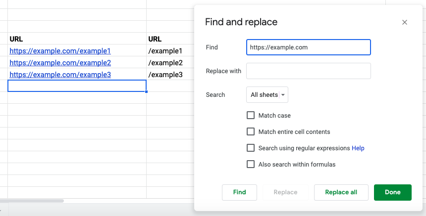
This means that all of your data is consistent an it took all of 10 seconds to do!
Other common application examples include:
- Replacing http with https
- Removing brand name from meta titles to be able to use the subject on its own
- Creating site structures by adding categories to URLs
- Replacing a commonly misspelled word in meta descriptions
- Fixing slightly incorrect results from a previous formula (if you forgot to add a space after full stops when merging columns, simply find “.” and replace with “. “)
- Removing unnecessary HTML if pages have been copied & pasted from Word (import to a text editor and get rid of stylings brought over from elsewhere)
The applications are endless and it should be a feature you go to without thinking about it. I can’t imagine working with data without the help of Find and Replace, it would take forever to conduct simple, menial tasks!If you are
3. Combine Text Values

This one is great for creating content en-masse. Whether that be formulating meta titles, meta descriptions or even entire page content. This formula will allow you to do that very efficiently.
Say you want to create a new value based on the combined information from a range of different columns, for a sheet of any more than 10 rows it would take forever to write it out manually. And it would take a lifetime to do it for sites with thousands of pages!
When Would You Need To Combine Text Values?
I find this one to be most common for e-commerce websites that have tens of thousands of products. Of course, in an ideal world every single product would have finely crafted unique text, but for the time vs outcomes doesn’t make any logical sense to do it this way.
Essentially, combining text values is useful for creating large amounts of formulaic content en-masse.
Multiple text values can be combined using a formula that looks like this:
=(“insert text”&CELL&”insert text”&CELL)
Here’s how that might look for e-commerce meta descriptions:

The end result will then look like this:

Of course, this is just an example to illustrate my point, meta descriptions need to be much longer than this and the wording isn’t exactly enticing – but you get the point.
I use this one all of the time and sometimes my formulas become so long and complex that it allows me to create super bespoke content in no time at all.
If you have lots more details you can use then you can craft really strong, tailored content en-masse. For example, you might also have product price, product dimensions, product colour, product category, or any number of unique pieces of information to make the text unique.
Quick tip: If you are applying these tips to an ecommerce store, you should also read my guide to the most common ecommerce site issues and how to fix them.
Another good application is to use this formula to create HTML en-masse such as generating links.
For example, if I want to create an HTML sitemap of hundreds of pages, I can create a formula to insert the URL and page name into the “a href” tag which can then be easily pasted into HTML editor of a page.
Whilst this is a real time-saver, it does get pretty complicated because the tag includes speech marks and so does the formula, meaning it looks a little like this:
=(“a href=”&”””&B2&”””&”>”&C2&”</a>”)
These applications take a little trial and error but the result is that you don’t have to do everything manually. If you’re still struggling to understand the formula, there’s a helpful guide on combining text values in Excel here.
4. Split Text To Columns Function

This is such an incredibly simple feature you can use in Google Sheets or Excel, and yet I’ve noticed that it is rarely used by beginners even though it only requires a few clicks of a button.
Splitting text to columns allows you to take a column of information and separate the contents into individual columns based on a defined delimiter. This means that you can then use one or more elements of the cell content for another purpose.
Simply highlight the column you wish you apply the formula to, click “Data” in the menu and then find “Split text to columns”. Options will appear asking you which delimiter you would like to split the text by. “Detect automatically” is quite often correct, but you can also use “Custom” to set your own.
When Would You Use Split Text To Columns?
Here’s an example of how Split text to columns is useful for SEO.
Say we have a list of meta titles that contain the product name, category name and the domain name. I would like to create meta descriptions based on these pieces of information so in order to use the use the function of combining text values (as described above), I first need to separate them into individual cells.
In this example, we have a range of t-shirts with unique colours and styles:
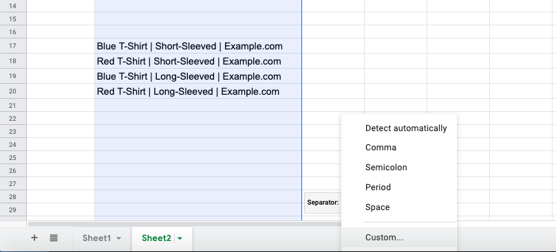
If we then set a custom delimiter of ” | ” and apply it, we then get each attribute in a separate cell which we can then begin to use how we wish.
As a result of this, we can now draft new formulas such as combining text values in order to create content that looks like this:

Again, it’s super simple but incredibly effective at saving time. Of course, you might want to fine-tune the results using other previously mentioned formulas. In this instance I added an “s” to T-shirt” in the formula but you could also use find and replace to add the S, or even to remove “.com” to just leave the brand name.
5. The Remove Duplicates Function

When working with mass amounts of data you will inevitably come up against duplicates for some reason or another.
Data doesn’t always come cleanly packaged how you would like it, and if you’re combining multiple sources of data then your odds of finding duplicates in your data is massively increased.
It’s relatively easy to remove duplicates manually, but if you’re working with thousands of rows of data it’s not a good use of your time to do it this way.
There are various ways to highlight or remove duplicate data in Excel or Google Sheets. However, the most simple way I have found to do this is to use the =UNIQUE(cell range) formula.
In order to apply the UNIQUE formula, simply start in a blank column and write out the formula =UNIQUE( then select the whole column of data, close brackets and press enter. Simple!
When Would You Need To Remove Duplicates?
With large data sets from multiple sources it is common to find large amounts of duplicates that are unnecessary for SEO purposes.
For example, many sites utilise URL parameters where additional pieces of information are added to a URL based on user activity such as filtering options on site, or tracking acquisition.
For SEO purposes, these are essentially the same URLs as you are unlikely to want to index each variation of a URL based on additional parameters. Therefore you will only need to edit information on the core URL and not each individual URL parameter.
In this scenario you can use functions such as text to columns to separate values that appear after a question mark, for example. Leaving you with a large amount of complete duplicate URLs.
You can then get rid of them all using the UNIQUE formula as follows:
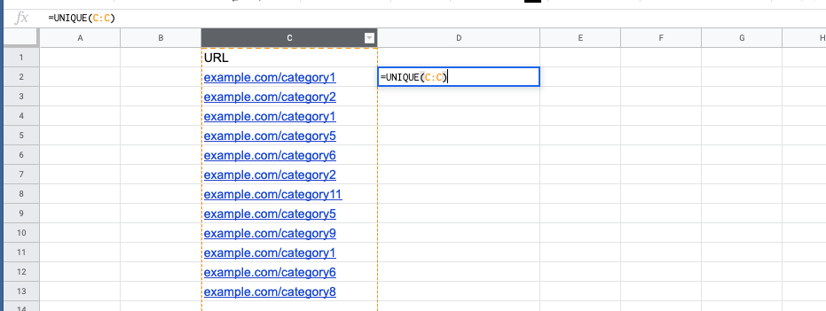
This gives you a much cleaner data set to work with and makes the job at hand much more straightforward.
6. The LEN Formula

The LEN formula is another one that is so gloriously simple and yet incredibly important for SEO specialists. The LEN formula very simply calculates the number of characters in a specified cell.
This allows you to determine whether the length of the contents within the cell is too long or short.
The LEN formula can be used by typing the following into a blank cell:
=LEN(insertcell)
…and pressing enter. (Of course, replace “insertcell” with the cell you would like to measure the length of). It should look a little like this:

You can then drag the formula down to find out which of your range is above or below the character length you are aiming for.

When Is The LEN Formula Useful For SEO?
Character count is important for many on-page elements for example:
- Meta titles
- Meta descriptions
- H1s
- Alt text
- Excerpts
If we know that the ideal meta title length for full optimisation is 50-60 characters, then we can pull a list of all meta titles, run the LEN formula and identify those that are either too long or too short.
The LEN formula then allows you to be able to identify quick wins very efficiently.
As an example, if you use this technique for meta descriptions, you will likely find a range of meta descriptions where the main keyword is at the end of a sentence that is far too long.
Whilst the keyword here isn’t a ranking factor, it can be very important for click through rate. So just spotting and fixing these can make a significant difference to your site’s traffic.
7. Conditional Formatting

Conditional formatting allows you to highlight (or format) cells that match a criteria that you have set. This means that you can spot values that are significant or visually display numbers based on whether they are positive or negative.
Conditional formatting is achieved by highlighting the column you’d like to use, clicking Format > Conditional Formatting and selecting your specification from within the sidebar.
You can choose to format cells based on a range of criteria such as “Greater than x”, “Less than x”, “In between x”, “Is equal to”, “Contains”, “Is empty” etc. This means your spreadsheet can be highly customised based on your set values.
When Would You Use Conditional Formatting?
I personally love conditional formatting for reporting. This allows me to visually display to my clients how traffic has increased month on month for pages or keywords in a way that allows them to judge immediately.
However, another amazing use is simply for spotting rows of data that don’t match your requirements. In the previous point about the LEN formula I discussed finding elements that are either too long or short to be well-optimised.
Conditional formatting allows you to identify these easily by colour coding those in green that are correct and those in red that need fixing. Applying conditional formatting in that instance would like a bit like this:
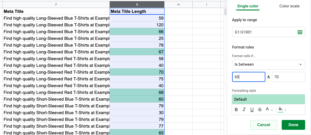
When you have thousands of rows of data, conditional formatting is a real time-saver. Of course, there are other methods for identifying certain ranges of data that match your criteria, but conditional formatting is quick, visual and effective.
Final Thoughts
Whether you’re an SEO Freelancer, an SEO Agency or an SEO beginner who has been put in charge of a company website, I hope these simple tricks make your life a lot easier!
In my recent article about SEO tips for nonprofits I spoke about conducting a top-level content audit to address duplicate content issues. By applying the data tips, you can turn a top-level content audit into an expert-level audit.
Of course, with bigger, more complex websites you will need to learn some much more advanced formulas but that can come later. I may even write a blog about the expert level formulas I use for SEO in the future.
Conversely, if you’re having some trouble figuring out how to optimise your website using data, do feel free to get in touch to discuss how I could help.


